Scaling vector search to billions of document chunks breaks traditional database architectures. Learn how to combine PostgreSQL 17 declarative HNSW partitioning in pgvector with Qdrant distributed segment optimization and single-stage hybrid metadata pre-filtering.

Executive Summary: The Vector Storage Scaling Wall at Billions of Chunks
In the early stages of Retrieval-Augmented Generation (RAG) and semantic search adoption (2023–2024), engineering teams operated under the illusion that vector databases were simply another key-value store. Indexing 100,000 to 1,000,000 document embeddings into a monolithic table was trivial. An in-memory Hierarchical Navigable Small World (HNSW) index constructed in milliseconds, and sub-10ms query latencies were achieved on modest cloud virtual machines.
By 2026, enterprise AI architectures have scaled to tens of millions of users, multi-tenant agentic memories, enterprise-wide codebase embeddings, and multimodal retrieval systems. At this scale, databases must index between 100 million and 10 billion high-dimensional vector embeddings ($d = 1536$ for OpenAI text-embedding-3-large or $d = 3072$ for frontier models).
At 1 billion 1536-dimensional vectors, monolithic database architectures hit a catastrophic physical scaling wall:
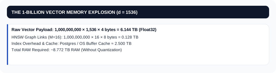
When an HNSW index exceeds available RAM, database operations degrade by orders of magnitude. The engine begins thrashing between SSD storage and memory, causing query latencies to spike from 8 milliseconds to over 3,200 milliseconds per nearest-neighbor search.
Furthermore, enterprise retrieval is almost never an unconstrained $k$-nearest neighbor search. Real-world enterprise queries mandate complex metadata pre-filtering (e.g., “Find chunks semantically similar to this prompt WHERE tenant_id = 'acme_corp' AND department = 'legal' AND created_at >= '2026-01-01' AND security_clearance <= 3”). Naive post-filtering drops recall to near-zero, while unindexed metadata scans exhaust database CPU cycles.
This comprehensive engineering guide breaks down the architectural blueprints for scaling vector search to billions of records. We explore PostgreSQL 17 declarative HNSW hierarchical partitioning in pgvector, deep-dive into Qdrant’s distributed Rust-native segment architecture with Scalar Quantization (SQ8), and solve the hybrid metadata search dilemma with single-stage bitmap pre-filtering.

pgvector vs. Qdrant: The Core Architectural Dilemma
When designing high-scale vector retrieval infrastructure, enterprise architects face a foundational trade-off: extend existing relational infrastructure with pgvector or deploy a purpose-built vector engine with Qdrant.
| Architectural Dimension | pgvector (PostgreSQL 17) | Qdrant (Rust Distributed Engine) |
|---|---|---|
| Underlying Storage Engine | PostgreSQL Heap + Buffer Manager | Custom Rust LSM-tree Segment Engine (mmap / NVMe) |
| Index Types Supported | HNSW, IVFFlat, Halfvec, Sparsevec (v0.8+) | HNSW with On-Disk Vector Storage & Inverted Payload Index |
| Vector Compression | Halfvec (FP16), Binary Quantization, 1-bit vectors | Scalar Quantization (SQ8), Product Quantization (PQ) |
| Metadata Filtering Execution | Iterative index scan (Postgres 16+) / Bitmap Join | Single-Stage Inverted Index Bitmap + Filtered HNSW Traversal |
| Partitioning & Sharding | Declarative Range/Hash Partitioning + Citus/CitusDB | Native Raft-based Horizontal Sharding & Collection Partitioning |
| Relational Joins & ACID | 100% Native ACID, Foreign Keys, Complex SQL Joins | Key-Value / Payload document storage (No SQL Joins) |
| Sweet-Spot Scale | 1M to 100M Vectors per Cluster | 10M to 10+ Billion Vectors in Distributed Clusters |
| Write / Ingestion Throughput | 5,000–15,000 vectors/sec (WAL bound) | 45,000–120,000 vectors/sec (Parallel segment streaming) |
The Decision Boundary
- Use pgvector when: Your dataset is under 100 million embeddings, strict ACID guarantees and relational foreign-key integrity are mandatory, and your team already possesses deep PostgreSQL operational expertise.
- Use Qdrant when: Your dataset exceeds 100 million embeddings, sub-10ms $p99$ latency is non-negotiable, write ingestion exceeds 20,000 records/sec, or you require advanced quantization with on-disk memory mapping to minimize cloud infrastructure costs.

Partitioning pgvector: PostgreSQL 17 Declarative HNSW Partitioning
In standard pgvector implementations, creating a single HNSW index across a table with 50 million rows results in a multi-gigabyte index file that must reside in PostgreSQL shared_buffers. Once multiple tenants query the table concurrently, cache eviction leads to catastrophic disk I/O thrashing.
The architectural solution is Declarative Hierarchical Partitioning using PostgreSQL 17's enhanced partition pruning engine.
The Mechanics of Partition Pruning for Vector Search
By partitioning the primary table along a deterministic boundary—such as tenant_id (Hash or List) or created_at (Range)—PostgreSQL creates separate, isolated physical tables for each partition. Crucially, each sub-partition builds its own localized HNSW index graph.
When a query includes the partition key in its WHERE clause:
- The PostgreSQL query planner immediately executes Static or Run-Time Partition Pruning.
- Unrelated partitions (and their multi-gigabyte HNSW index graphs) are completely bypassed.
- The query scans only the localized HNSW graph of the targeted partition, reducing graph traversal depth from $O(\log N_{\text{total}})$ to $O(\log N_{\text{partition}})$.
- The localized index fits entirely within RAM / L3 cache, eliminating disk reads.MERMAID
graph TD
Query[Incoming Semantic Query: WHERE tenant_id = 'tenant_42'] --> Planner[PostgreSQL 17 Query Planner]
Planner --> Prune{Partition Pruner}
Prune -.->|Skip 99% of Data| Part1[Partition 00: HNSW Graph - BYPASSED]
Prune -.->|Skip 99% of Data| Part2[Partition 01: HNSW Graph - BYPASSED]
Prune ==>|Direct Scan| Part42[Partition 42: Local HNSW Graph]
Part42 --> Result[Top-K Nearest Neighbors in <6ms]
Production PostgreSQL 17 DDL: Hierarchical Partitioned pgvector Table
-- Enable vector extension (pgvector v0.8.0+)
CREATE EXTENSION IF NOT EXISTS vector;

-- Create parent partitioned table by tenant_id hash
CREATE TABLE document_embeddings (
    id UUID NOT NULL,
    tenant_id VARCHAR(64) NOT NULL,
    document_id UUID NOT NULL,
    chunk_index INT NOT NULL,
    metadata JSONB NOT NULL,
    embedding VECTOR(1536) NOT NULL,
    created_at TIMESTAMPTZ NOT NULL DEFAULT NOW(),
    PRIMARY KEY (tenant_id, id)
) PARTITION BY HASH (tenant_id);

-- Create 16 discrete hash partitions for horizontal distribution
CREATE TABLE document_embeddings_p00 PARTITION OF document_embeddings
    FOR VALUES WITH (MODULUS 16, REMAINDER 0);
CREATE TABLE document_embeddings_p01 PARTITION OF document_embeddings
    FOR VALUES WITH (MODULUS 16, REMAINDER 1);
CREATE TABLE document_embeddings_p02 PARTITION OF document_embeddings
    FOR VALUES WITH (MODULUS 16, REMAINDER 2);
-- (... partitions p03 through p15 created similarly ...)

-- Build localized HNSW indexes on each individual partition
-- Parameters: m=16 (max connections per node), ef_construction=128 (construction search width)
CREATE INDEX idx_embeddings_p00_hnsw ON document_embeddings_p00
USING hnsw (embedding vector_cosine_ops) WITH (m = 16, ef_construction = 128);

CREATE INDEX idx_embeddings_p01_hnsw ON document_embeddings_p01
USING hnsw (embedding vector_cosine_ops) WITH (m = 16, ef_construction = 128);

-- Create GIN index for high-performance JSONB metadata pre-filtering
CREATE INDEX idx_embeddings_p00_meta ON document_embeddings_p00 USING gin (metadata);
CREATE INDEX idx_embeddings_p01_meta ON document_embeddings_p01 USING gin (metadata);
Optimized Partition-Pruned Query Execution
To guarantee that PostgreSQL activates partition pruning, always parameterize queries with the exact partition key:
-- Set runtime search width (ef_search controls latency vs recall)
SET hnsw.ef_search = 64;

-- Query hits ONLY partition 42 with zero cache pollution
EXPLAIN ANALYZE
SELECT id, document_id, 1 - (embedding <=> '[0.012, -0.043, ... 1536 dims]') AS cosine_similarity
FROM document_embeddings
WHERE tenant_id = 'tenant_enterprise_42'
  AND (metadata->>'department') = 'legal'
ORDER BY embedding <=> '[0.012, -0.043, ...]'
LIMIT 10;
Qdrant Cluster Topology: Dynamic Segment Rebuilding and Index Tuning
While pgvector is ideal for relational-bound workloads, scaling past 100 million vectors requires a distributed, memory-efficient engine. Qdrant achieves billion-scale retrieval through its unique Segment-Based Storage Architecture written in Rust.
The Anatomy of a Qdrant Segment
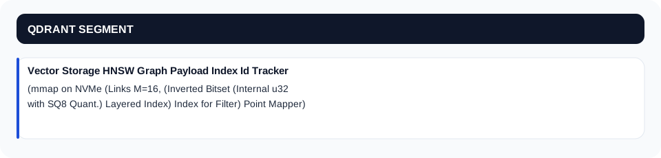
In Qdrant, a collection is split into multiple Segments. Each segment is an independent, self-contained search index consisting of:
- Vector Storage: Raw vectors stored in memory or memory-mapped (
mmap) directly from NVMe SSDs. - HNSW Graph: Multi-layer proximity graph linking points within that specific segment.
- Payload Index: Inverted index mapping metadata fields (keywords, integers, geo-coordinates, booleans) to bitsets for instant boolean evaluation.
- Id Tracker: Bi-directional mapping between external point IDs and internal sequential 32-bit indices.
Dynamic Segment Lifecycle: WAL $\to$ Mutable $\to$ Immutable $\to$ Optimized
To maintain high write throughput without degrading search performance, Qdrant executes a continuous segment lifecycle:
- Ingestion into Mutable Segment: New vectors and payloads are appended to an in-memory mutable segment and simultaneously flushed to the Write-Ahead Log (WAL).
- Sealing & Freezing: When the mutable segment reaches a threshold (e.g., 200,000 points or 256 MB), it is sealed, becoming Immutable.
- Background Optimization & Merging: A background daemon merges small immutable segments into large, highly optimized segments. During this merge, deleted points (tombstones) are purged, HNSW graph connections are re-balanced, and Scalar Quantization (SQ8) is computed.
- Zero-Downtime Hot Swapping: The newly built segment atomically replaces the older segments with zero read interruption.
Quantization: Reducing 6 TB RAM Footprint by 75%
To conquer the vector storage scaling wall, Qdrant utilizes Scalar Quantization (SQ8). SQ8 converts 32-bit floating-point numbers (Float32, 4 bytes per dimension) into 8-bit integers (UInt8, 1 byte per dimension) based on the statistical distribution of each vector coordinate:
$$\tilde{x}_i = \text{round}\left( 255 \times \frac{x_i - \min_i}{\max_i - \min_i} \right)$$
Combined with on_disk: true for original unquantized vectors, Qdrant stores the 8-bit quantized vectors in RAM for ultra-fast SIMD distance calculations during initial candidate search, streaming the full-precision vectors from NVMe disk only for the final top-$k$ re-ranking stage.
Result: Memory consumption drops from 6.14 TB to 1.53 TB RAM with a negligible recall loss ($<0.005$ drop in Recall@10).

Co-Located Hybrid Queries: Solving the Metadata Filtering Dilemma
In real-world enterprise applications, vector search without metadata filters is virtually useless. However, combining unstructured vector proximity with structured metadata predicates presents one of the hardest challenges in database theory.
The Collapse of Naive Post-Filtering
In naive vector databases, the engine executes a standard $k$-nearest neighbor search first (e.g., retrieving the top 100 closest vectors globally) and then applies metadata filters (e.g., WHERE tenant_id = 'acme').
The Failure: If the tenant represents only 0.1% of the total dataset, the top 100 global results may contain zero records belonging to that tenant. The database returns an empty result set despite thousands of valid matching documents existing in the database. Oversampling ($k=10,000$) causes massive latency spikes and memory exhaustion.
Single-Stage Hybrid Pre-Filtering (The Qdrant & pgvector Solution)
To achieve 100% recall with sub-10ms latency, modern engines implement Single-Stage Filtered HNSW Traversal:
- Payload Bitset Generation: Before traversing the vector graph, the engine evaluates the metadata filter using in-memory inverted indices, generating an ultra-compact bitset representing all valid point IDs.
- Filtered Graph Traversal: During the HNSW graph traversal, when evaluating neighboring candidate nodes, the engine executes a bitwise
ANDcheck against the payload bitset using CPU hardware SIMD instructions. - Graph Skipping / Custom Entry Points: If a subgraph has low density, the engine dynamically falls back to an exact vector scan over the payload-filtered subset, guaranteeing that valid results are never missed.MERMAID
sequenceDiagram
autonumber
actor Client as AI Agent / Application
actor Engine as Qdrant Hybrid Query Router
participant Inverted as Payload Inverted Index
participant HNSW as Filtered HNSW Traversal
participant Storage as On-Disk Rescorer (NVMe)

Client->>Engine: Search(Vector, Filter: dept='legal' AND year>=2025)
Engine->>Inverted: 1. Evaluate Filter Condition
Inverted-->>Engine: 2. Return In-Memory Point Bitset (0b1011001...)
Engine->>HNSW: 3. Traverse HNSW with Bitmask Validation
HNSW-->>Engine: 4. Candidate Top-100 Quantized IDs (RAM)
Engine->>Storage: 5. Exact Full-Precision Re-Rank (Top-10)
Storage-->>Client: 6. Return Top-10 Valid Documents in 6.4ms

Distributed Sharding & High Availability
When scaling to 1 billion vectors across a cluster, high availability and horizontal query distribution require a multi-node cluster topology.
Qdrant Distributed Architecture
- Stateless Query Routers: Ingress gateways that receive gRPC/REST search requests, determine which shards hold relevant data based on the tenant partition key, scatter the query across cluster nodes in parallel, and merge/re-rank the top-$k$ results.
- Raft Consensus Group: Manages cluster state, shard routing tables, and collection schemas with zero external dependencies (no Zookeeper or Etcd required).
- Physical Shard Replicas (Replication Factor = 3): Each partition is replicated across three distinct physical availability zones. Read queries are dynamically routed to the replica with the lowest CPU load and queue depth.
Production Implementation: Async Python Qdrant Engine with Hybrid Metadata Filtering
The following production-ready Python service demonstrates how to initialize a quantized, partitioned Qdrant collection, ingest high-dimensional vectors with structured payloads, and execute sub-10ms hybrid pre-filtered searches:
"""
Enterprise Billion-Scale Vector Retrieval Service (2026).
Implements Qdrant Async Client with Scalar Quantization (SQ8),
on-disk vector storage, and single-stage hybrid metadata pre-filtering.
"""

import asyncio
import uuid
from typing import List, Dict, Any, Optional
from qdrant_client import AsyncQdrantClient
from qdrant_client.http import models


class ScaledVectorSearchEngine:
    def __init__(self, host: str = "localhost", port: int = 6334) -> None:
        self.client = AsyncQdrantClient(host=host, port=port, prefer_grpc=True)
        self.collection_name = "enterprise_knowledge_base"

    async def initialize_optimized_collection(self, vector_dim: int = 1536) -> None:
        """
        Configures collection with on-disk vectors, SQ8 quantization,
        and optimized HNSW graph parameters for billion-scale retrieval.
        """
        collections = await self.client.get_collections()
        exists = any(c.name == self.collection_name for c in collections.collections)

        if not exists:
            await self.client.create_collection(
                collection_name=self.collection_name,
                vectors_config=models.VectorParams(
                    size=vector_dim,
                    distance=models.Distance.COSINE,
                    on_disk=True  # Stream raw float32 vectors from NVMe
                ),
                # Configure in-memory 8-bit Scalar Quantization (SQ8)
                quantization_config=models.ScalarQuantization(
                    scalar=models.ScalarQuantizationConfig(
                        type=models.ScalarType.INT8,
                        quantile=0.99,
                        always_ram=True  # Keep compressed vectors in RAM for SIMD
                    )
                ),
                # Optimize HNSW Graph connectivity
                hnsw_config=models.HnswConfigDiff(
                    m=16,
                    ef_construct=128,
                    on_disk=False  # Keep graph in RAM for maximum traversal velocity
                ),
                # Configure multi-node horizontal sharding
                shard_number=6,
                replication_factor=3
            )

            # Create inverted payload indexes for instant metadata pre-filtering
            await self.client.create_payload_index(
                collection_name=self.collection_name,
                field_name="tenant_id",
                field_schema=models.PayloadSchemaType.KEYWORD
            )
            await self.client.create_payload_index(
                collection_name=self.collection_name,
                field_name="department",
                field_schema=models.PayloadSchemaType.KEYWORD
            )
            await self.client.create_payload_index(
                collection_name=self.collection_name,
                field_name="security_clearance",
                field_schema=models.PayloadSchemaType.INTEGER
            )
            print(f"Collection '{self.collection_name}' initialized with SQ8 and inverted indexes.")

    async def upsert_embeddings_batch(
        self,
        records: List[Dict[str, Any]]
    ) -> None:
        """Batch upsert points with vector and structured payload metadata."""
        points = [
            models.PointStruct(
                id=str(uuid.uuid4()),
                vector=rec["vector"],
                payload={
                    "tenant_id": rec["tenant_id"],
                    "document_id": rec["document_id"],
                    "department": rec["department"],
                    "security_clearance": rec["security_clearance"],
                    "text_chunk": rec["text_chunk"],
                    "created_at": rec["created_at"]
                }
            )
            for rec in records
        ]

        await self.client.upsert(
            collection_name=self.collection_name,
            points=points,
            wait=False  # Async background flush to WAL for maximum throughput
        )

    async def execute_hybrid_prefiltered_search(
        self,
        query_vector: List[float],
        tenant_id: str,
        department: str,
        max_clearance: int,
        limit: int = 10
    ) -> List[Dict[str, Any]]:
        """
        Executes single-stage hybrid search: Inverted index pre-filter +
        SIMD HNSW traversal + on-disk exact rescore.
        """
        # Define strict metadata pre-filter
        search_filter = models.Filter(
            must=[
                models.FieldCondition(
                    key="tenant_id",
                    match=models.MatchValue(value=tenant_id)
                ),
                models.FieldCondition(
                    key="department",
                    match=models.MatchValue(value=department)
                ),
                models.FieldCondition(
                    key="security_clearance",
                    range=models.Range(lte=max_clearance)
                )
            ]
        )

        search_results = await self.client.search(
            collection_name=self.collection_name,
            query_vector=query_vector,
            query_filter=search_filter,
            limit=limit,
            search_params=models.SearchParams(
                hnsw_ef=64,
                exact=False,
                quantization=models.QuantizationSearchParams(
                    rescore=True  # Rescore top candidates with full precision from disk
                )
            )
        )

        return [
            {
                "id": hit.id,
                "score": hit.score,
                "payload": hit.payload
            }
            for hit in search_results
        ]
The 3-Step Monday Morning Action Plan: Scaling Your Vector Architecture
Ready to optimize your vector database for enterprise scale? Execute this practical roadmap:
Step 1: Profile Your Vector-to-RAM Ratio (Week 1)
Calculate your current memory consumption: $\text{Vectors} \times \text{Dimensions} \times 4 \text{ bytes}$. If your unquantized vector index consumes more than 50% of available database RAM, immediate intervention is required. In pgvector, switch to halfvec (FP16) or declarative table partitioning. In Qdrant, enable scalar_quantization (SQ8).
Step 2: Implement Partition Pruning on pgvector (Week 2)
Convert monolithic PostgreSQL embedding tables into declarative hash or range partitions by tenant_id. Verify that your application queries include the partition key in all WHERE clauses, and run EXPLAIN ANALYZE to confirm that unused partitions are pruned.
Step 3: Build Inverted Payload Indexes Before Vector Reindexing (Weeks 3–4)
Never perform metadata filtering on unindexed JSONB or payload fields. In PostgreSQL, build GIN indexes on your JSONB metadata columns. In Qdrant, create explicit keyword and integer payload indexes to enable hardware-accelerated single-stage hybrid pre-filtering.
Frequently Asked Questions (FAQ)
1. Why does an HNSW index fail when vector counts exceed available RAM?
An HNSW index is an interconnected multi-layer proximity graph. When traversing the graph to find nearest neighbors, the query engine makes frequent random-access memory hops across nodes. If the graph cannot fit into RAM, every graph hop triggers a physical disk read from storage. This random disk I/O causes query latency to explode from less than 10 milliseconds to over 3,000 milliseconds per query.
2. How much RAM does Scalar Quantization (SQ8) save compared to full precision?
Scalar Quantization (SQ8) converts 32-bit floating-point numbers (4 bytes per coordinate) into 8-bit unsigned integers (1 byte per coordinate). This delivers an immediate 75% reduction in vector memory footprint. Combined with on-disk full-precision storage for final top-k rescoring, SQ8 allows a single node to store 4x more embeddings with less than 0.5% recall loss.
3. What is the difference between Pre-Filtering and Post-Filtering in vector search?
Post-filtering searches the global vector graph first and removes non-matching metadata rows afterward, which causes severe recall drop if the filtered subset is small. Pre-filtering evaluates metadata first using an inverted index bitset, ensuring that the vector traversal only inspects valid candidates. Single-stage hybrid pre-filtering combines both steps during graph traversal, achieving 100% recall with ultra-low latency.
4. When should I choose pgvector over a dedicated vector database like Qdrant?
Choose pgvector when your dataset is under 100 million embeddings, your application requires strict ACID transactions and relational SQL joins with existing business tables, and you want to avoid managing separate database infrastructure. Choose Qdrant when scaling past 100M to billions of vectors, when write throughput exceeds 20,000 vectors/sec, or when memory-mapped quantization is needed to reduce infrastructure costs.
5. How does PostgreSQL 17 improve pgvector performance?
PostgreSQL 17 enhances query plan optimization for declarative partitioning, improves parallel worker utilization during index builds, and integrates seamlessly with pgvector 0.8+ features like iterative index scans, SIMD-accelerated distance functions (AVX-512 and ARM NEON), and half-precision (halfvec) vectors.
6. Can I shard a pgvector database across multiple physical servers?
Yes. You can scale pgvector horizontally across multiple PostgreSQL nodes using extensions like Citus Data (distributed PostgreSQL) or by deploying application-level tenant sharding where each physical PostgreSQL instance maintains a subset of tenant partitions.
Structural Schema Markup (JSON-LD)
LINKEDIN_HOOK: Architectural blueprint for scaling vector search to billions of embeddings.
